$if(mathjax)$ $endif$

Artificial Intelligence.

In this space we will address issues related to Artificial Intelligence, in the book Artificial Intelligence a Modern Approach, written by Staiart Russell and Peter Norving divides the concepts into four possible areas such as: Systems that think like humans, Systems that think rationally, systems that acts like humans, systems that act rationally.[1]

Machine Learning

Occurence Probability

The approach to data analysis is based on the mean of the distribution represented by the next equation, which is the standard form of the Gaussian distribution [2]. \begin{equation} P(x) = \frac{1}{\sqrt{2 \pi \sigma ^2}} e^{\frac{x - \mu }{2 \sigma ^2}} \end{equation} Where $P(x)$ is the probability of occurrence of the variable n, $\sigma$ is the Standard deviation, $\sigma$ 2 is the Variance, $\mu$ is the Mean. The method is based on the postulate that the values of the unknown parameters are those that produce a maximum probability of observing the measured data. Assuming that the measurements are independent of each other [2].

Data distribution

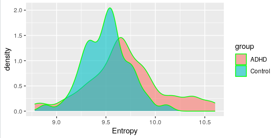
The following code shows how to make a graph on the density distribution of the data, it is understood that it is the calculated entropy of the electroencephalogram signals of a subject diagnosed with Attention Deficit Disorder and Control subjects.

library(ggplot2)
#Name     label  
#Control  <- 0 
#ADHD     <- 1    

file1 <-"Desktop/Ingoodwetrust/libros/ADHD_dataset_2/var_st_entropy_AP_RP_Control_ADHD_V2_1.csv"
df1 <- read.csv(file1)

file0 <-"Desktop/Ingoodwetrust/libros/ADHD_dataset_2/var_st_entropy_AP_RP_Control_ADHD_V2_0.csv"
df0 <- read.csv(file0)

g1 <- replicate(265,"ADHD")
g2<- replicate(265,"Control")

df1$group <- g1 
df0$group <- g2
df <- rbind(df1,df0)

df$Entropy <- df$entropy

p2 <- ggplot(df, aes(x=Entropy, fill=group, binwidth=.3)) + geom_density(col = "green", alpha=.6) 

p2

The following graph shows the distribution density of the data.

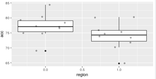
After running the algorithm 10 times, we can see in the following figure the comparison between two algorithms, the one proposed in this chapter and Logistic Regression, which is defined by region 1.0.

Linear Regression

The simple linear regression model, is a model with a single regressor x that has a relationship with a response y that is a straight line, we can found this equations in the book Introduction to linear regression Analysis [3]. \begin{equation} y_0 = \beta_0 + \beta_1 x_0 \end{equation} where the intercept $\beta_0$ and the slope $\beta_1$ are unknown constants.

References.

[1] Stuart Russel, Peter Norving . (2004). Artificial Intelligence a Modern Approach. 28042 Madrid (España): Pearson Education,.

[2] M. Bonamente, Statistics and Analysis of Scientific Data. Springer Science+Business Media New York 2013, 2013.

[3] Douglas C. Montgomery. (2012). Introduction to Linear Regression Analysis. Hoboken, New Jersey.: John Wiley & Sons, Inc

Capter 2

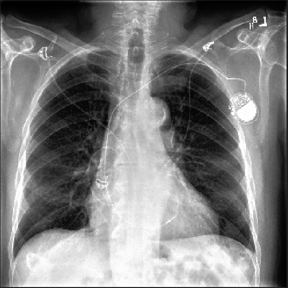
Chest X ray

Datasets

Publics datasets CheXpert, NIH and Covid19.

Classes Weights.

It can be seen that the database is not balanced, that is, the diference between the number of classes is very high, for this reason, the loss function BCEWithLogitsLoss is used, and their weights are calculated respectively with the following equation:

\begin{equation}
pos_weight = \frac{N}{P} \end{equation}

where N are negative examples an P positives examples.

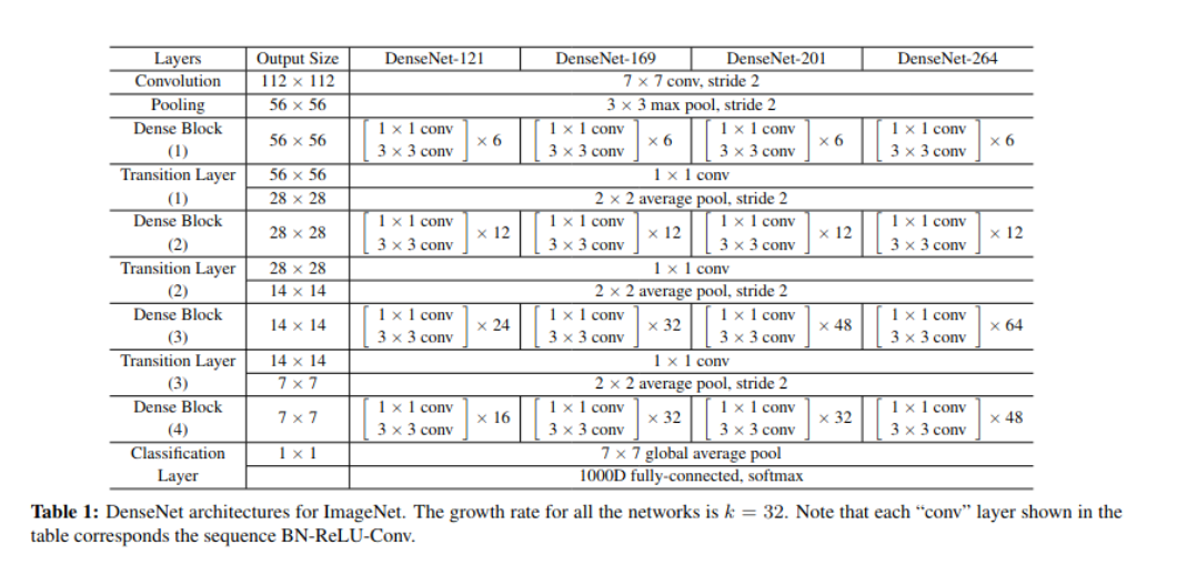
DenseNet 121.

Error metrics.

One of the problems faced is dealing class imbalanced, that is, when one of the classes is outnumbers than the other classes [10], to deal with this problem, the followed metrics are used: Weighted Average Precision, Weighted Average Recall, Fβ and Weighted Average Specificity.

Weighted Average Precision.

\begin{equation}
WeightedAveragePrecision = \frac{|y_i|}{|y|} * Precision_1 + \frac{|y2|}{|y|}*Precision_2 \end{equation}

Weighted Average Recall (Sensitivity).

\begin{equation}
WeightedAverageRecall = \frac{|y_i|}{|y|} * Recall_1 + \frac{|y2|}{|y|}*Recall_2 \end{equation}

F_beta.

\begin{equation}
WeightedAveragef1score = \frac{|y_i|f1score_1}{|y|} + \frac{|y2|f1score_2}{|y|} \end{equation}

Weighted Average Specificity.

\begin{equation}
WeightedAveragespecificity = \frac{|y_i|}{|y|} * Specificity_1 + \frac{|y2|}{|y|}*Specificity_2 \end{equation}

Capter 3

Violence Detection.

Datasets

Hockey fight Dataset, Movies Dataset, Violent-Flow Dataset.

Deep Learning Model.

AlexNet-LSTM.

The convolution layers were trained to extract features from the video frames and then be encapsulated using a convLSTM layer, the neural network works as follows: The frames of the videos under consideration are sequentially applied to the model. Once all the frames are applied, the hidden state of the convLSTM in the final step contains the representation of the input video frames. The video representation, in the hidden state of the convLSTM, is applied to a series of fully-connected layers for classification [3].

In the proposed model, is used the AlexNet model [4], pre-trained on the ImageNet database as the CNN model for extracting frame level features [3]. In the convLSTM, was used 256 filters in all the gates with a filter size of 3 x 3 and stride 1. Thus the hidden state of the convLSTM consist of 256 feature maps. A batch normalization layer is added before the first fully-connected layer. Rectified linear unit (ReLU) non-linear activation is applied after each of the convolutional and fully-connected layers. The network is trained to minimize the binary cross entropy loss [3].

Error metrics

Precision

\begin{equation}
Precision = \frac{TP}{Tp+Fp} \end{equation}

Recall (Sensitivity).

\begin{equation}
Recall = \frac{TP}{Tp+Fn} \end{equation}

F_beta.

\begin{equation}
f_1score = \frac{2∗Precision∗Recall}{Precision+Recall} \end{equation}

Specificity.

\begin{equation}
Specificity = \frac{Tn}{Tn+Fp} \end{equation}

Accuracy

\begin{equation}
Accuracy = \frac{Tp + Tn}{Tp + Tn + Fp + Fn} \end{equation}

$if(mathjax)$ $endif$